The unbearable effectiveness of the Central Limit Theorem

The Central Limit Theorem is one of the most astonishing results in statistics. Let’s cover briefly what it states (in one of its forms): if we have \(N\) independent and identically distributed random variables that come from a distribution (that we will call the underlying distribution) with mean \(\mu\) and variance \(\sigma^2\), then the average of those variables will, as \(N\) increases, resemble a normal distribution centered in \(\mu\) with variance \(\sigma^2/N\). We can even replace \(\sigma^2\) with the sample variance \(S^2\) and the CLT still holds.¹

And let’s cover, just for clarity, what it’s not: the CLT does not say that the distribution of \(X_i\) will be normal, and it does not say that the standard deviation of the distribution will be reduced as we draw more variables. This might seem obvious when you’re reading it in context and thoughtfully, but it is a source of confusion in a lot of discussions about the CLT, so it’s worth keeping in mind.

But there is one more thing that the CLT does not say, a critical one for practitioners of data science, statistics and the likes: when will I have enough \(N\)? Even more: how do I even know I have enough \(N\)? We will try to answer these questions analyzing first a scenario in which the math is relatively easy and well-known and taking advantage of the exact results to draw general conclusions.

Start small: the underlying distribution is Normal

If the underlying distribution were normal and we knew the variance we are in the presence of a very specific result in which the average is normally distributed for every sample size, even from \(N=2\). This involves doing some math to find that the sum of two normal variables is normal and then calculating the average dividing by \(N\).

So let’s start with something that at least involves an approximation, right? Suppose we knew that the underlying distribution is Normal but, unlike the previous case, now we don’t know the variance. In this case, instead of using \(\sigma^2\) we can use the sample variance \(S^2\). Because of this we don’t expect the average to be exactly normally distributed, but we do expect it to tend to a normal distribution as \(N\) increases.

Although not as much as before, we are still lucky! The distribution of the average for this case can be calculated analytically. It was done more than 100 years ago by William Gosset, and it’s the famous t-distribution.² To compare the distribution of the averages with the expected normal from the CLT, we’ll do something very usual: standardizing the variable. If we expect \(\bar{X}\) to have a distribution \(\mathcal{N}(\mu, S^2)\) we can standardize \(\bar{X}\) by substracting \(\mu\) and dividing by \(S\) so that, in the regime of the Central Limit Theorem,

To check how good our approximation is, then, we just have to calculate this standardized variable and see how it compares with the standard normal distribution. In the following figure we’ve plotted the Cumulative Density Function for the t-distribution for \(N=2\), \(N=10\), \(N=30\) and \(N=100\) samples and compare it with the CDF of the normal distribution.

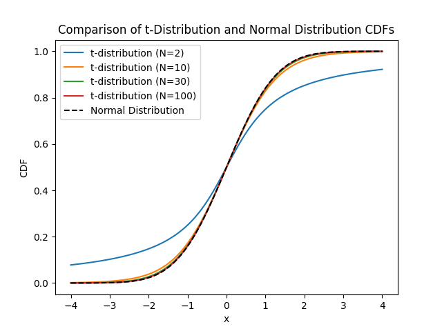
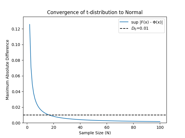
It’s clear that, as \(N\) increases, the distributions start to look more like the standard normal.³ We are almost there, we need only one more thing: try to quantify when it’s good enough. We could choose a lot of different ways to measure it, but we have to pick one. Arbitrarily⁴ we pick the Kolmogorov distance, defined as the maximum of the absolute value of the differences between our CDF and the standard normal, \(D = \text{sup}\left\|F(x) - \Phi(x)\right\|\).

So this is how we are going to analyze the distributions similarity to the Normal distribution:

1. For every value of \(x\) we will calculate the distance between our CDF and the standard normal,
2. Then pick the maximum among all of these \(x\), this will be the Kolmogorov distance.
3. We’ll use this value to compare how “similar” the CDF is to the standard normal.
4. We will set an arbitrary threshold \(D_0 = 0.01\) for “practical” convergence⁵.

In our case for the t-distribution, this is reached at \(N_c=18\).

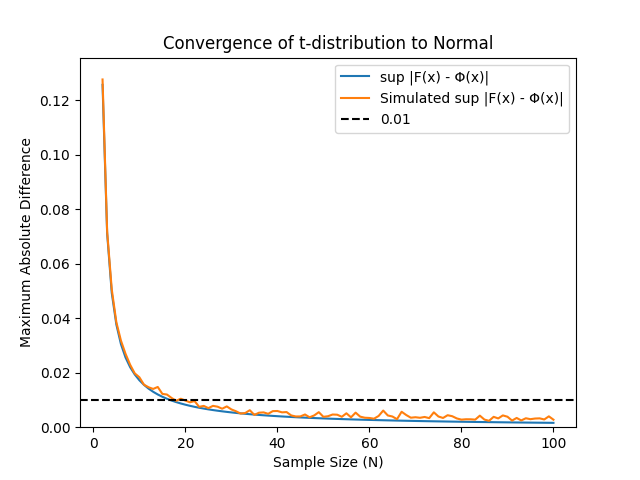
We are almost there, we need to add only one more ingredient to the mix: what will we do when we don’t have exact results? In this case, we will have to rely on simulations⁶.

An unknown result: the underlying distribution is binomial

OK, we have everything we need! Now we can do our analysis for every distribution, let’s try first the binomial. We will use the same strategy as before and now calculate the \(N_c\) at \(D_0 = 0.01\) as a function of the probability \(p\).

Again, remember the idea: we compare the CDF of the average with the standard normal, calculate the maximum difference for different sample sizes \(N\) and see when it’s below our threshold of \(D_0 = 0.01\). This will be the critical sample size, \(N_c\). Unlike the previous case, here we expect \(N_c\) to depend on the underlying probability, so in the following figure we plot \(N_c\) as a function of \(p\).

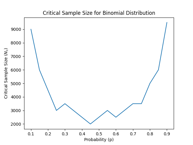
Of course this is a noisy plot because the simulations take time and we can’t be as fine-grained as we wish⁷. Therefore we have a very coarse sampling of \(p\) and the sample sizes. But I hope you get the core idea: first of all, that the critical sample size depends on the underlying distribution and that, even for the same underyling distribution, it might vary a lot depending on its parameters. Nonetheless, we can see that the critical sample size is not that large when compared to the amount of data we are used to in most data science applications.

What can I do with an unknown distribution?

But let’s face it: the most common scenario is that we don’t know the underlying distribution. After all, if we knew it we could just infer the parameters with a technique like Maximum Likelihood Estimation and then calculate the mean of the distributions for the parameters. Or, if we were doing a hypothesis test, simply do a Likelihood Ratio Test. There is however an approach you can take: from all of the data you have, bootstrap \(N\) samples and use the simulations we’ve just made to calculate \(D\) for each of them. This will give you an idea of the sample size you need to approximate your distribution to a normal one.

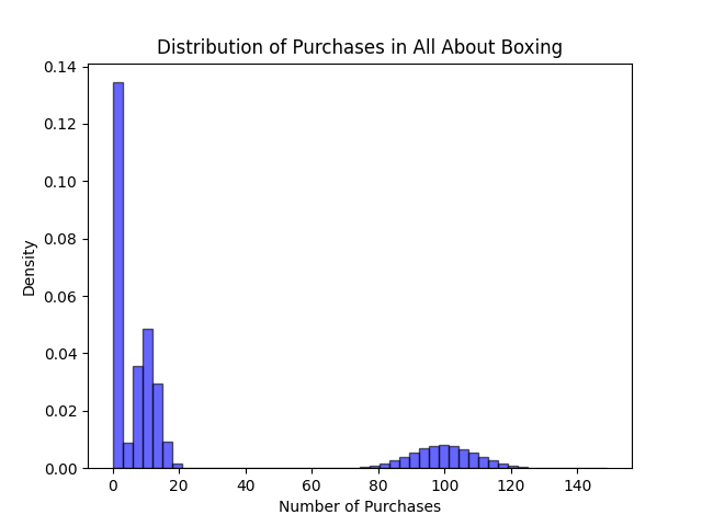
Just as an example, suppose we are data scientists in All About Boxing, a company that sells cardboard boxes online. Our users will, with probability \(p_0\), buy nothing. With probability \(p_1\) they will buy from a Poisson distribution with mean 10 and, with probability \(p_2\) they will buy from a Poisson distribution with mean 100. This is roughly what the distribution would look like:

Before you go on reading, test your intuition! How many samples would you say we need for this model to comply with our threshold of \(D_0=0.01\). My guess (I haven’t run it yet!) is around \(N=1000\). Now let’s plot \(D\) as a function of \(N\):

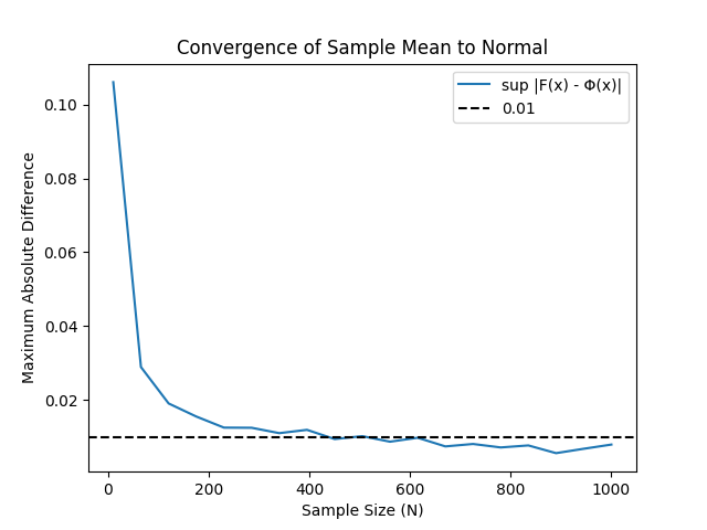
I admit I’m surprised! I was being aggressive with \(N=1000\), but it looks as even \(N=500\) should be enough. To be honest, this result not only is suprising, but it also feels… demoralizing. One of the fun parts of statistics is the actual modelling of the underlying distribution, we’d love to take the empirical distribution of All about boxing and try to guess what’s the underlying distribution that fits best. This result shows that in some scenarios, when we are interested in estimating the mean of the distributions, we don’t need to go that far. This happens particularly in AB tests for online experiments (these have the characteristic that the sample size tends to be relatively large). For data scientists that spend quite some time analyzing AB tests the effectiveness of the Central Limit Theorem is unbearable: it renders useless some of the fun parts of statistics.

Don’t despair though: there are still a lot of challenging problems statistics-wise for AB tests, even using the CLT: sequential testing, effect size estimation, multiple comparisons, and many more. We will cover these topics in future posts, stay tuned.